Parabolic Shot
m (Somes of the screenshots needs to be updated with 0.64.0) |
m (Text replace - "{{Category|NewTerminology}}" to "{{NewTerminology}}") |
||
| Line 3: | Line 3: | ||
{{Category|Tutorials}} | {{Category|Tutorials}} | ||
{{Category|Tutorials Advanced}} | {{Category|Tutorials Advanced}} | ||
| − | {{ | + | {{NewTerminology}} |
<!-- Page info end --> | <!-- Page info end --> | ||
Somes of the screenshots needs to be updated with 0.64.0 | Somes of the screenshots needs to be updated with 0.64.0 | ||
Revision as of 10:01, 20 May 2013
Somes of the screenshots needs to be updated with 0.64.0
This is a small tutorial to show how to make an object follow a path given by a mathematical function, as requested here.
Contents
Mathematical function to follow
We're going to simulate a cannon shot. A cannonball describes a parabolic trajectory after it is fired from the cannon.
The mathematical equations that govern the trajectory are:
Failed to parse (MathML with SVG or PNG fallback (recommended for modern browsers and accessibility tools): Invalid response ("Math extension cannot connect to Restbase.") from server "https://api.formulasearchengine.com/v1/":): {\displaystyle X(t)=V_{0x}\cdot t+X_0}
Failed to parse (MathML with SVG or PNG fallback (recommended for modern browsers and accessibility tools): Invalid response ("Math extension cannot connect to Restbase.") from server "https://api.formulasearchengine.com/v1/":): {\displaystyle Y(t)=-\frac{1}{2}\cdot G \cdot t^2 + V_{0y}\cdot t + Y_0}
where:
Failed to parse (MathML with SVG or PNG fallback (recommended for modern browsers and accessibility tools): Invalid response ("Math extension cannot connect to Restbase.") from server "https://api.formulasearchengine.com/v1/":): {\displaystyle t} = the current time for the mathematical equation.
Failed to parse (MathML with SVG or PNG fallback (recommended for modern browsers and accessibility tools): Invalid response ("Math extension cannot connect to Restbase.") from server "https://api.formulasearchengine.com/v1/":): {\displaystyle X} = the 'x' coordinate of the bullet at a time 't'
Failed to parse (MathML with SVG or PNG fallback (recommended for modern browsers and accessibility tools): Invalid response ("Math extension cannot connect to Restbase.") from server "https://api.formulasearchengine.com/v1/":): {\displaystyle Y} = the 'y' coordinate of the bullet at a time 't'
Failed to parse (MathML with SVG or PNG fallback (recommended for modern browsers and accessibility tools): Invalid response ("Math extension cannot connect to Restbase.") from server "https://api.formulasearchengine.com/v1/":): {\displaystyle X_0} = the 'x' position of the bullet at time t = 0
Failed to parse (MathML with SVG or PNG fallback (recommended for modern browsers and accessibility tools): Invalid response ("Math extension cannot connect to Restbase.") from server "https://api.formulasearchengine.com/v1/":): {\displaystyle Y_0} = the 'y' position of the bullet at time t = 0
Failed to parse (MathML with SVG or PNG fallback (recommended for modern browsers and accessibility tools): Invalid response ("Math extension cannot connect to Restbase.") from server "https://api.formulasearchengine.com/v1/":): {\displaystyle V_{0x}} = the 'x' component of the velocity when shot (t = 0)
Failed to parse (MathML with SVG or PNG fallback (recommended for modern browsers and accessibility tools): Invalid response ("Math extension cannot connect to Restbase.") from server "https://api.formulasearchengine.com/v1/":): {\displaystyle V_{0y}} = the 'y' component of the velocity when shot (t = 0)
Failed to parse (MathML with SVG or PNG fallback (recommended for modern browsers and accessibility tools): Invalid response ("Math extension cannot connect to Restbase.") from server "https://api.formulasearchengine.com/v1/":): {\displaystyle G} = the gravity's acceleration.
You usually have the angle and the velocity modulus instead of its components. The decomposition is quite easy:
Failed to parse (MathML with SVG or PNG fallback (recommended for modern browsers and accessibility tools): Invalid response ("Math extension cannot connect to Restbase.") from server "https://api.formulasearchengine.com/v1/":): {\displaystyle V_{0x} = V_0 \cdot \cos \varphi}
Failed to parse (MathML with SVG or PNG fallback (recommended for modern browsers and accessibility tools): Invalid response ("Math extension cannot connect to Restbase.") from server "https://api.formulasearchengine.com/v1/":): {\displaystyle V_{0y} = V_0 \cdot \sin \varphi}
where:
Failed to parse (MathML with SVG or PNG fallback (recommended for modern browsers and accessibility tools): Invalid response ("Math extension cannot connect to Restbase.") from server "https://api.formulasearchengine.com/v1/":): {\displaystyle V_0} = the velocity when shot (t = 0)
Failed to parse (MathML with SVG or PNG fallback (recommended for modern browsers and accessibility tools): Invalid response ("Math extension cannot connect to Restbase.") from server "https://api.formulasearchengine.com/v1/":): {\displaystyle \varphi} = the cannon shooting angle with the horizontal.
See this Wikipedia article if you need more information regarding the maths equations of a parabolic shot.
Converting the functions
So, how can you introduce these functions into Synfig? To do that you must convert the function from infix (e.g. 3 + 2) to prefix (e.g. + 3 2) notation.
Once decomposed then you realize how many independent variables you need for the simulation. Also you will discover what are the 'engines' for the animation and what are parameters.
Let's start with the X coordinate:
Failed to parse (MathML with SVG or PNG fallback (recommended for modern browsers and accessibility tools): Invalid response ("Math extension cannot connect to Restbase.") from server "https://api.formulasearchengine.com/v1/":): {\displaystyle X=V_{0x}\cdot t+X_0}
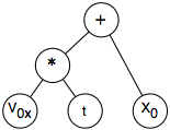
Using the common arithmetic precedence rules (multiplication and division are higher precedence than addition and subtraction) the function can be decomposed as:
- The addition of two terms: (V0x*t) + (X0)
- The first term is a multiplication of two single terms: (V0x) * (t)
- And the third term is a single term (X0)
So to convert those formula into a Synfig understandable way you should create the following conversion types (between parentheses are the conversion types and between brackets are the exported values or the current values if not exported:
- [X] (Add)
- LHS [X0]
- RHS [X0] (Scale)
- Link [V0x]
- Scalar [t]
- Scalar [1.0]
(Notice that the Scalar parameter from the Add convert type is not used so its value is 1.0)
So with this conversion type X becomes X0+(V0x*t).
Let's continue with the Y coordinate:
Failed to parse (MathML with SVG or PNG fallback (recommended for modern browsers and accessibility tools): Invalid response ("Math extension cannot connect to Restbase.") from server "https://api.formulasearchengine.com/v1/":): {\displaystyle Y=-\frac{1}{2}\cdot G \cdot t^2 + V_{0y}\cdot t + Y_0}
This one is a little more complicated because there are more terms. Anyway you should always try to group the terms in pairs and see what operator is used. Take care on the arithmetic operators properties (commutative, associative, distributive and identity) to respect the final values of the formulae. We will search for the operators with the lower order of precedence (multiplication, division and modulus precede addition and subtraction).
So there are two '+' operators what gives three terms: (-0.5*G*t²) + (V0y*t) + (Y0). Then since Synfig has only a two term convert type for addition operation, we need to make the Add conversion twice.
Continuing with the analysis, the individual terms are composed by multiplied terms: (-0.5) * (G) * (t²) and (V0y) * (t).
The same problem arises again; Synfig has a conversion type called 'Scale' that gives the multiplication of a Link by an Scalar. So we need to make the Scale conversion several times for the first term (in fact three times due to the fact that t²=t*t), and once for the second term.
So the final result is this:
- Y (Add)
- LHS (Scale)
- Link (Scale)
- Link (Scale)
- Link [t]
- Scalar [t]
- Scalar [G]
- Link (Scale)
- Scalar [-0.5]
- Link (Scale)
- RHS (Add)
- LHS (Scale)
- Link [V0y]
- Scalar [t]
- RHS [Y0]
- Scalar [1.0]
- LHS (Scale)
- Scalar [1.0]
- LHS (Scale)
Now let's study the velocity composition with the velocity modulus and its shooting angle.
Failed to parse (MathML with SVG or PNG fallback (recommended for modern browsers and accessibility tools): Invalid response ("Math extension cannot connect to Restbase.") from server "https://api.formulasearchengine.com/v1/":): {\displaystyle V_{0x} = V_0 \cdot \cos \varphi}
Failed to parse (MathML with SVG or PNG fallback (recommended for modern browsers and accessibility tools): Invalid response ("Math extension cannot connect to Restbase.") from server "https://api.formulasearchengine.com/v1/":): {\displaystyle V_{0y} = V_0 \cdot \sin \varphi}
You can see that splitting these formulae is very simple once you have understood what Synfig needs:
- V0x (Cos)
- Angle [phi]
- Amplitude [V0]
and
- V0y (Sin)
- Angle [phi]
- Amplitude [V0]
OK I've analysed the maths functions but how do I put them into Synfig?
Well, in the example of the cannon and ball, I've assigned the X and Y values to the X and Y values of the centre of the circle that defines the bullet. You can assign the mathematical equations to any of the convertible parameters that exist in any layer.
Go to the circle Center parameter, right click, and select 'Convert -> Composite' from the context menu. Once done you'll obtain two sub-parameters: 'X-axis' and 'Y-axis'.
Right click on the corresponding parameter that you obtain after each convert type and select the correct conversion type from the analysis you have done before. Then you will convert sequentially each sub-parameter to the proper one.
Once done you should export the most simple terms to allow easy modification or reuse. For example, the t variable (the time for the mathematical equation) is used in more than one place. You should export it only once. The rest of the times that t appears you should select the exported t Valuenode from the Library Panel, right click and 'Connect' to reuse it.
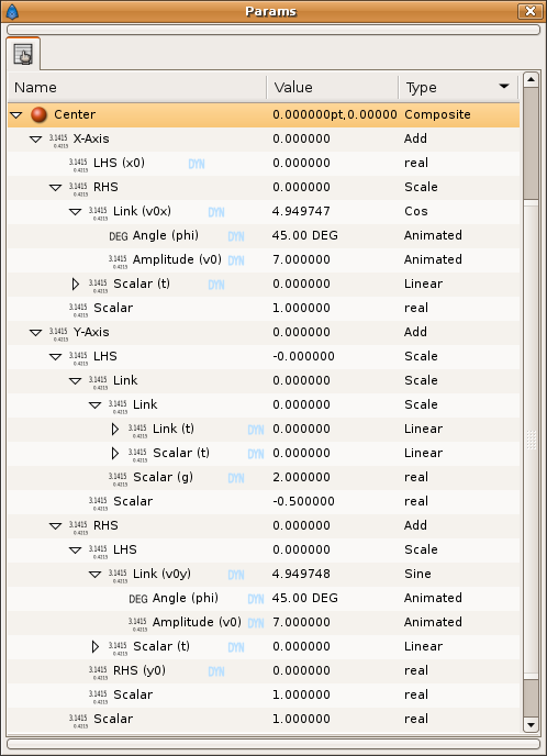
Once done you should obtain something like this:
The t parameter
In this case the 'engine' of the equations is the variable t (the physics time). To make the engine parameter to 'move' in the animation we need to link it to the animation's current time. To do that we will use the 'Linear' convert type. In fact this one is the only conversion that allows a parameter to change with the animation time.
The 'Linear' conversion gives two sub-parameters:
Rate: amount of change of the converted parameter in one second of animation time.
Offset: value to add to the result of the multiplication of the animation time by the Rate value.
So if the converted type is t we will obtain:
t = Rate*T + Offset
where T is the current animation time in seconds.
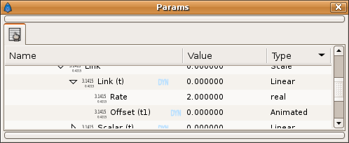
You should have notice that in the image of the conversion types result, the t parameter is also converted. It was not expanded in order not to complicate the sample. Here is the result:
I've exported the Offset parameter as t1 to allow easy manipulation during the animation.
Setting up the parameters
Once done all the conversions and all the exportations you can go to the Library Panel ValueNode list and insert the proper values for the parameters of the animation: V0, phi, G, X0, Y0, t1
The X-axis and Y-axis parameters are calculated based on the variation of the 't' parameter that is linear with the animation time T. You can also export the parameter 'Rate' form the converted type 't' if you want extra external variation of the equation motion. Test the values of the mentioned animation parameters to the desired ones. Specially some combinations of G and V0 gives good or bad values. I've set G=2.0 so my example is not in the earth :)
Producing more than one shot
You have notice that the shot animation is a little boring due to it starts at time T=0 and there is only one shot. How can you do the same than the sample? How can I use the same bullet several times making different shots with different angles, positions and initial velocities? Quite easy. Use the Offset parameter form the Linear conversion of the 't' variable.
Initially the Offset parameter is set to 0.0. That means that t=T or in other hands, the animation time is the same than the equation time. But what happen if you modify the Offset parameter during the animation?. You can 'rewind' the equation motion to the place you want just inserting the proper values of the Offset parameter at the proper animation time.
| T (sec) | Offset (t units) | Rate (t units/sec) | t = Rate*T+Offset | Offset waypoint (in/out) |
| 0.0 | 0.0 | 2.0 | 0.0 | linear/linear |
| 0.5 | -1.0 | 2.0 | 0.0 | linear/linear |
| 4.0 | -8.0 | 2.0 | 0.0 | constant/linear |
| 5.5 | -11.0 | 2.0 | 0.0 | linear/linear |
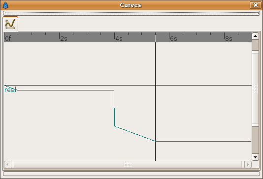
Those are the graphical representation for the above values:
Offset curve:
Rate curve:
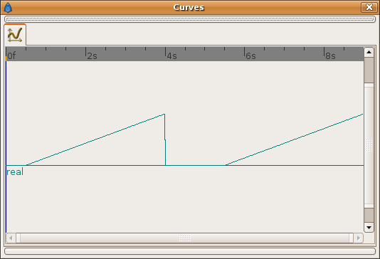
't' curve:
Notice that between T=0 and T=0.5 the Offset value has a linear variation that is inverse to the current Rate (2.0). It produces a no variation on the 't' parameter.
Also when Offset is set to constant = -1.0 (between T=0.5 and T=4.0 seconds) the 't' curve becomes linear (according to the value of Rate). During that period of time the equation is in 'action' and the parabolic shot is done with the current values of X0, Y0, V0, phi and G.
When Offset is suddenly set to -8.0 at T=4.0 it produces a 'rewind' of the equation animation to its 'zero' (t=Rate*T+Offset=2.0*4.0-8.0=0.0) so the bullet comes again to its origin.
Notice again that between T=4 and T=5.5 the Offset parameter has a linear variation between -8.0 and -11.0 (what comes from the current T value, divided by the Rate and changed sign), what gives a 't' result constant and equal to 0.0.
Again, from T=5.5 and beyond, the Offset is set to constant (there is no waypoint later so the value is kept) and the 't' value becomes linear (again there is a second shot). But in this case at T=5.5 the other parameters have been set to other different values (angle is higher and initial velocity is lower) using a constant waypoint. It allows to simulate a new shot with different parameters.
The file link and other comments
The above animation can be found also at youtube. The result sifz file for that animation is here.
I've added a fancy shooting cannon (it has a rotation angle linked to the 'phi' parameter) a motion blur on the bullet and some background.
I hope you enjoyed the tutorial. If need any help please ask it in any of the usual places.


