Doc:Ball Bounce
This is a tutorial to explain how to create a bounce tutorial. The main target of the tutorial covers the ball movement. It is known that cartoon like balls have also a very deformed poses meanwhile thery are travelling and speciphically when it hits the ground. This could be covered in a second stage.
Different aproximations for the same result
With Synfig there are four ways to create a bounce ball using the technical posibilities of this program.
- The first one is do the bounce ball manually. That would involve create several waypoints and adjust them to match a parabolic movement (in time and in path).
- Second way is use the interpolations paramters of the waypoints when they are set to TCB interpolation. This would drastically reduce the amount of waypoints and also make easier the timing of the bounces.
- Third way to perform a bounce ball is make use of the Link to bline abiliity. If you draw the path of a bouncing ball using a bline it is quite easy to make the ball follow the path even changing the bouncing speed.
- The fourth way to simulate a bouncing ball is create the mathematical equations to do that. Just make several parabolic shots at the rigth place a the right time to simulate a bouncing ball. It would be a little tricky but probably should be the most accurate one.
Manual Ball Bounce
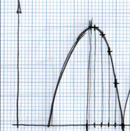
The rule to make the ball bounce manually is to draw in a paper the desired bounce. Then mark the horizontal line with regular intervals and match the curve intersection in vertical. See the image:
You can notice that having regular intervals in the horizontal axis gives irregular intervals to the vertical axis. It is due to the nature of the curve.
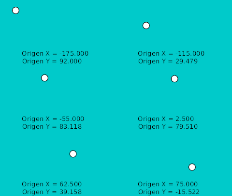
Once the points are located in a 2D grid then it can be drawn directly in Synfig doing use of the grid (F11). After draw them I normalized the values to be completely symmetrical. That gives the following table:
| Time | X position | Y position | Comments |
| 0f | -175.0 | 92.0 | Highest point |
| 4f | -165.0 | 92.0 | |
| 8f | -155.0 | 81.118 | |
| 12f | -145.0 | 63.678 | |
| 16f | -135.0 | 29.479 | |
| 20f | -125.0 | -15.522 | Lower point |
| 24f | -115.0 | 29.479 | |
| 28f | -105.0 | 63.782 | |
| ... | ... |
You can see that the X position is increasing in steps of 10.0 and the Y position reproduces a parabolic curve.
To proceed with more than one bounce just duplicate the waypoints (place the cursor at the right place right click over the waypoint and duplicate) reproducing symmetrical movements. You should need to edit the X values manually to decrease by 10.0 for each new waypoint.
The resulting animation and file is this one.
File: Media:manual.sifz
Ball Bounce using waypoints interpolations
The TCB interpolation mode allows modify the Tension, Continuity, Bias, and Temporal Tension values of the waypoint. So you can create easily smooth or peak aproximation to the value of the valuenode in the wypoint position.
This time I would use the same values for the highest and lower points of the table before. But I won't use more than one waypoint for each extreme position. The rest of the curve would be done using the TCB parameters.
That's the resulting animation:

